Disentanglement != Axis Alignment

Last updated on Jul 8, 2020 7 min read

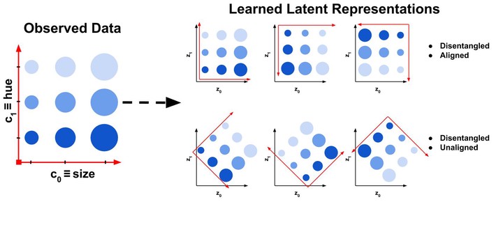Illustration of how a disentangled manifold can be both aligned and unaligned with the basis vectors.

TL;DR - The bottleneck layer of a VAE might be disentangled, up to a rotation, which might make it look entangled upon the standard visual inspection following a linear latent axis interpolation. An additional PCA step could be all one needs.

Preface

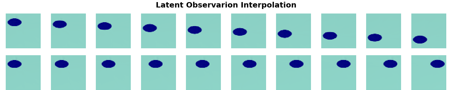
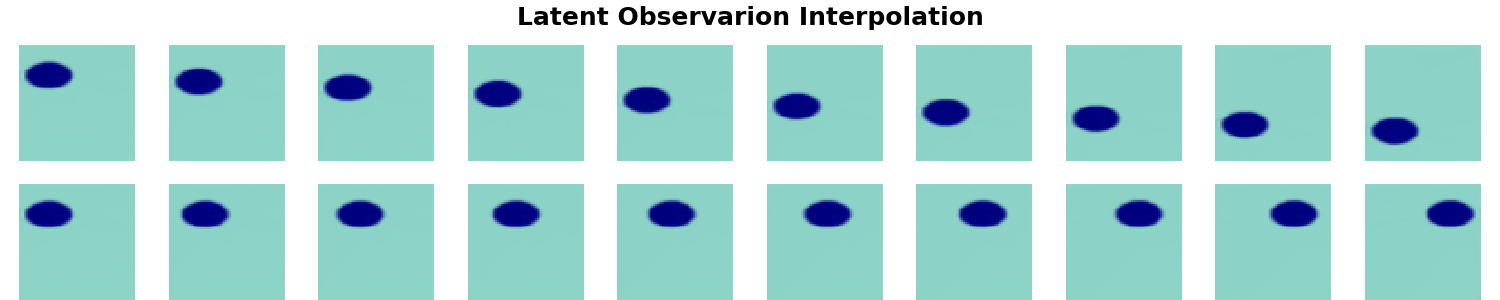
There are multiple metrics, scores and frameworks in the existing literature which can be used to get a quantitative measure of how disentangled a given vector space $\mathbf{z}$ is. More concretely, the vector spaces $\mathbf{z}$ considered in the context of achieving disentanglement are usually the bottleneck layer of a deep generative latent variable model - e.g. a VAE. When the model is trained on image data, often an additional visual qualitative evaluation is used - each of the standard basis vectors spanning $\mathbf{z}$ are linearly perturbed around the origin and the reconstructed images corresponding to the series of latent perturbations are inspected as to whether they contain isolated factors of variation - abstract notions and concepts we'll call $\mathbf{c}$.

Concisely, the latent space $\mathbf{z}$ of a VAE is deemed disentangled if a set of conceptually-orthogonal notions $\mathbf{c}$ are contained as a set of orthogonal vectors in $\mathbf{z}$. For example, in the image above, the notions of object size ($c_o$) and object color ($c_1$), which are conceptually-orthogonal (independent of each other), are contained in $\mathbf{z} \in \mathbb{R}^{2}$ as a pair of orthogonal vectors. Another good and visually-supported example is this recent tweet by David Pfau below:

"Disentangling" is a somewhat nebulous term in ML, but it is broadly about building models that can separate out different latent factors of variation - for instance, in vision, separating translation, rotation, and changes in lighting or color that leave objects invariant. 2/n pic.twitter.com/w9viBryx9D
— David Pfau (@pfau) June 24, 2020

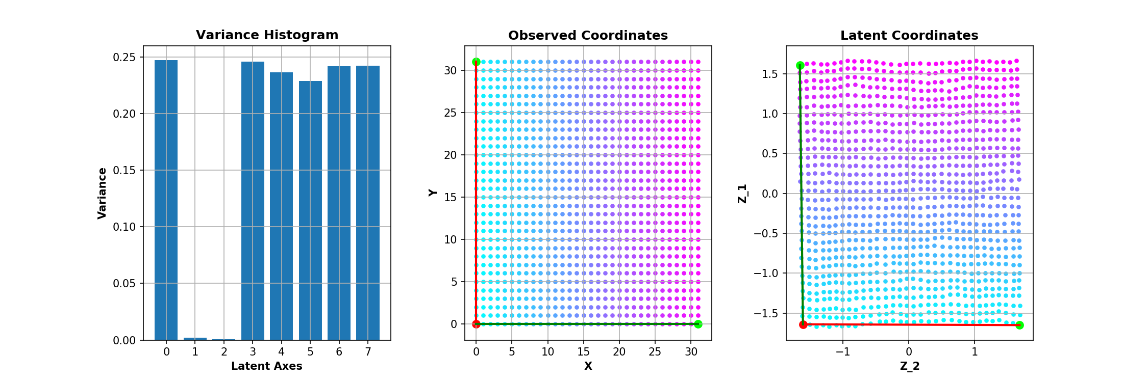
While intuitive, there's a major assumption in that form of visual evaluation which has been emphasized in a paper by Watters et. al - the assumption that the factors of variation $\mathbf{c} = \{$x pos, y pos, size, color$\}$ align with the standard basis spanning $\mathbf{z}$. By alignment here we mean that there is a one-to-one correspondence between individual factors of variation and the basis vectors of the latent space. As demonstrated in the paper, and below, this is not necessarily always the case.

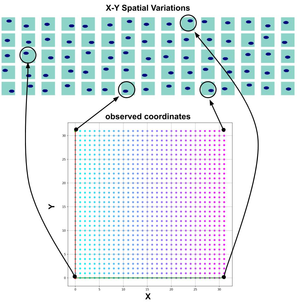
Positional Variations

All experiments are aimed at reproducing some of the results from the Spatial Broadcast Decoder paper by Watters et. al. Since we want to have neat visualisations we constrain ourselves to 2D. All the data that we use is a modification of the Deepmind dSprites dataset. In the first example we have an image of a single ellipse whose X and Y positions can vary - 32 possible values for each. The X and Y position variations are the conceptually orthogonal notions $\mathbf{c} = \{c_0, c_1\}$, implicitly contained in the image pixels.

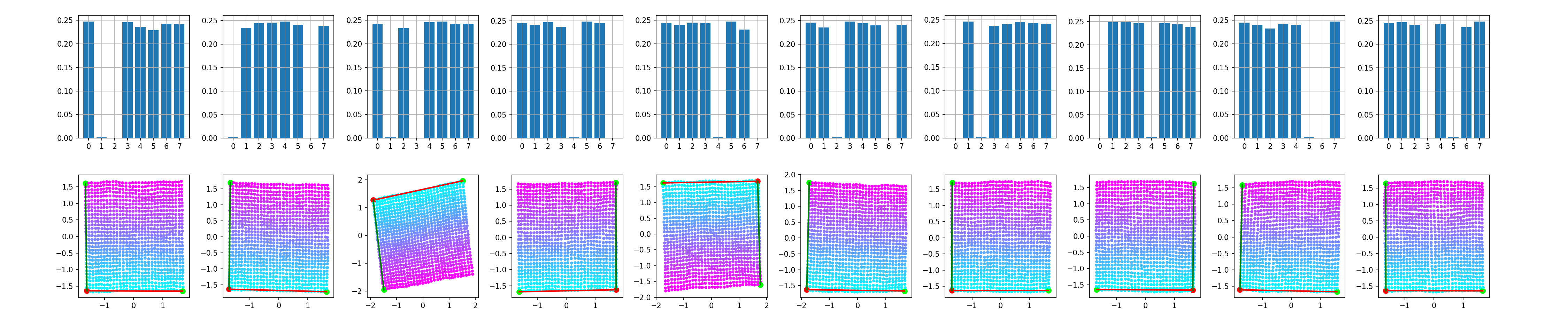
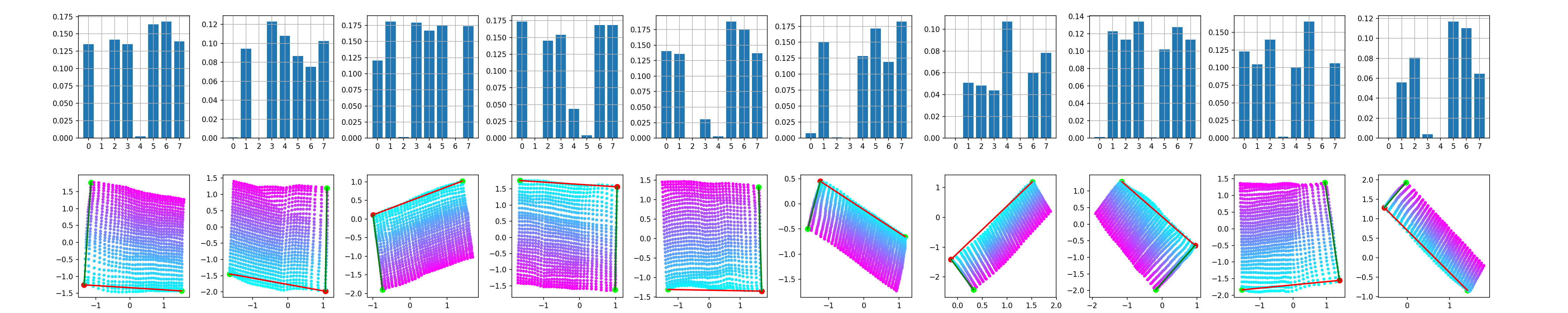
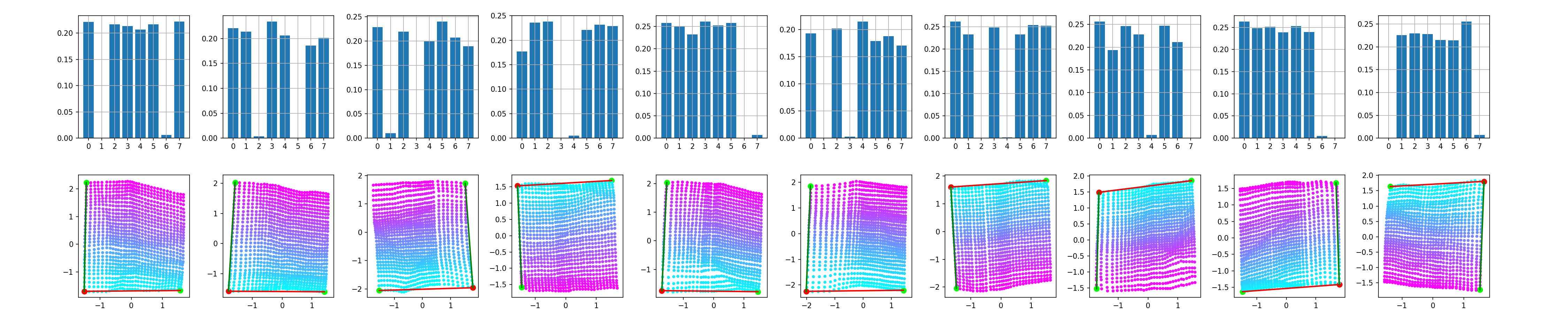
Data with two factors of variation - $c_0 \equiv$ X-position (32 values, green line) and $c_1 \equiv$ Y-position (32 values, red line) of the ellipse; **(top)** random samples from **(bottom)** the uniform distribution over $\mathbf{c}$

The trained model is a convolutional $\beta$-VAE with a spatial broadcast decoder and size for the latent space $|\mathbf{z}|$ = 8 - example implementation here. The question is whether we can have any 2 out of the 8 dimensions of $\mathbf{z}$ to be equivallent to $\mathbf{c}$. This is inspected in the following manner - after training, all the images are encoded and the two dimensions with smallest average variance predictions are identified as good candidates for encoding $\mathbf{c} = \{c_0, c_1\}$, following the rationale of the original paper.

$\beta$ = 1

Interpolating the 2 basis vectors with smallest average predicted var - $z_0$ and $z_2$ - in the range [-2,2]; **(row 1)** perturbing $z_0$ corresponds to changes in both X and Y position; **(row 2)** perturbing $z_2$ corresponds to changes in both X and Y position;

Interpolating the latent projections of $c_0$ and $c_1$ - red and green lines above; **(row 1)** perturbing red line corresponds to changes only in Y position; **(row 2)** perturbing green line corresponds to changes only in X position;

Results from 10 different experiments. Variance histograms & latent projections of $\mathbf{c}$ are shown.

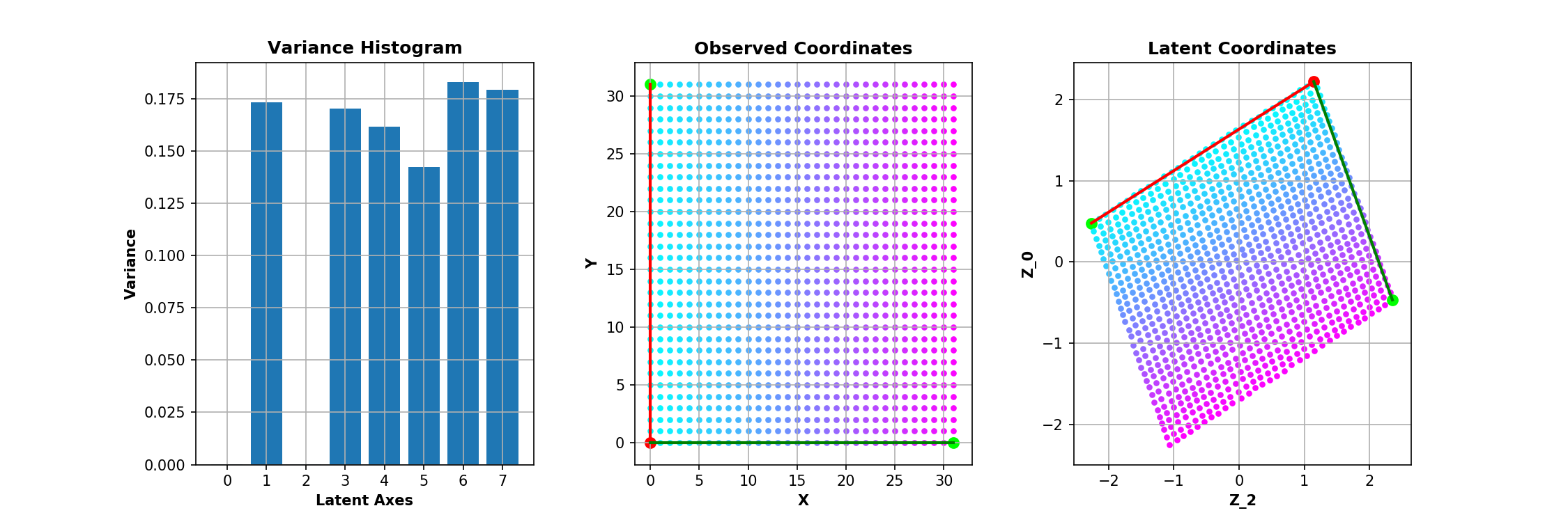
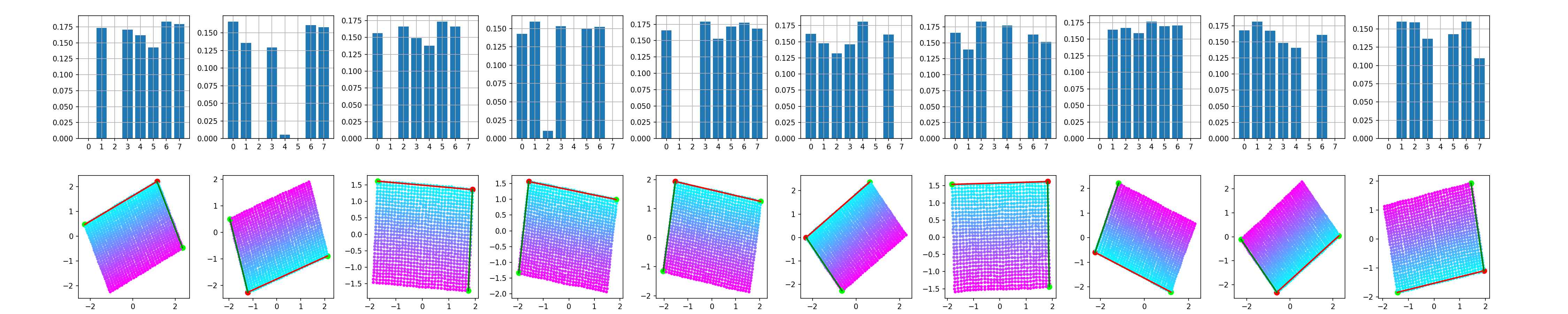
The same experiment is repeated 10 times. It is interesting to see that even though the bottleneck layer of the VAE is consistently disentangled - the square of observed values for the factors of variation is preserved as such in the latent space - it is often unaligned - the square is rotated. It is worth noting that the 2D subspace of $\mathbf{z}$ representing $\mathbf{c}$ is so nicely disentangled mainly due to the inductive biases the model has - i.e. the spatial broadcast decoder (as discussed in the original paper). However, that's a topic for future post, axis alignment is what we focus on here.

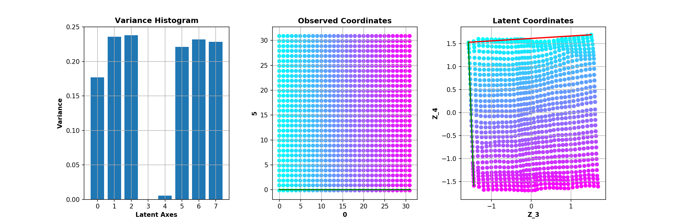
$\beta$ = 10

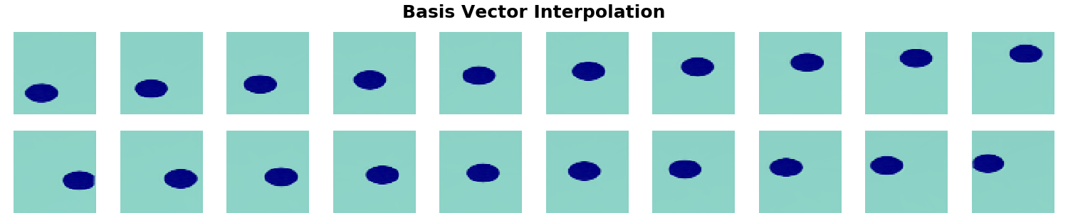
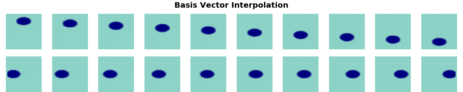
One way to account for the observed rotation of the learned representations is by tuning the coefficient of the KL divergence in the loss and enforcing more independce between the latent vectors $\mathbf{z}$. For the keen, there are examples in the literature for more principled ways of enforcing such constraints - e.g. 1 and 2. As seen below, increasing $\beta$ does lead to more consistent disentanglement and alignment - perturbing the basis vectors of $\mathbf{z}$ and the latent projections of $\mathbf{c}$ contain the same conceptual information.

Interpolating the 2 basis vectors with smallest average predicted var - $z_1$ and $z_2$ - in the range [-2,2]; **(row 1)** perturbing $z_2$ corresponds to changes only in Y position; **(row 2)** perturbing $z_1$ corresponds to changes only in X position;

Tuning coefficients of separate terms in the optimised loss function, like $\beta$, can be very case-by-case and dataset-specific.

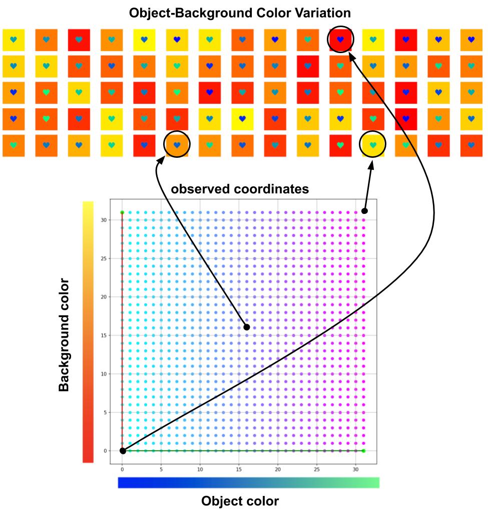
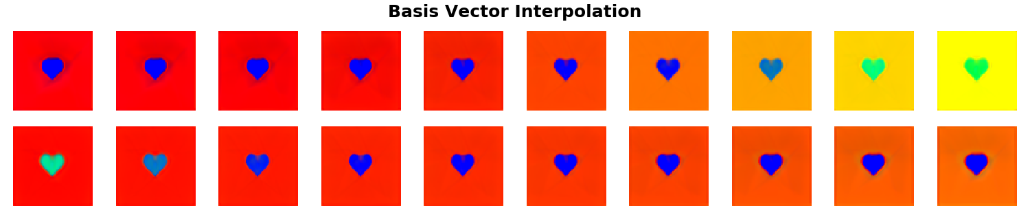
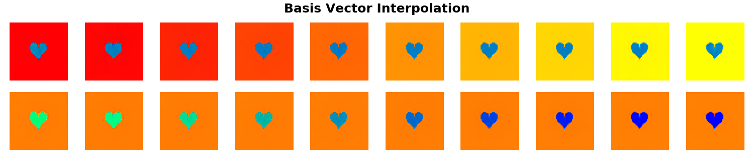
Color Variations

The data used in the two experiments above contains only spatial variations for which the Spatial Broadcast Decoder was specifically designed. Out of interest we repeat the same two experiments, but this time with data that has no spatial variations, only color-based ones.

Data with two factors of variation - $c_0 \equiv$ Object color (32 values, green line) and $c_1 \equiv$ Background color (32 values, red line); **(top)** random data samples from **(bottom)** the uniform distribution over $\mathbf{c}$

In the following two experiments instead of $\beta$ we explore how does the length of training affect the learned representations.

Epochs = 100; $\beta$ = 1

Example results for a **disentangled** but **unaligned** representation after training a $\beta$-VAE ($\beta$=1) for 100 epochs; rest is the same as above.

Interpolating the 2 basis vectors with smallest average predicted var - $z_0$ and $z_5$ - in the range [-2,2]; **(row 1)** perturbing $z_0$ corresponds to changes in both background color and object color; **(row 2)** perturbing $z_5$ corresponds to changes in both background color and object color;

Interpolating the latent projections of $c_0$ and $c_1$ - red and green lines above; **(row 1)** perturbing red line corresponds to changes only in background color; **(row 2)** perturbing green line corresponds to changes only in object color;

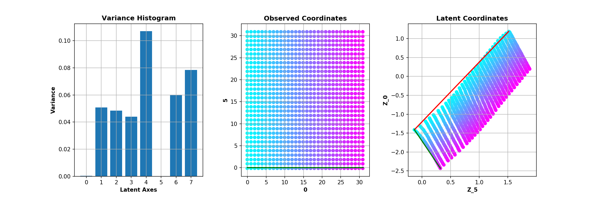
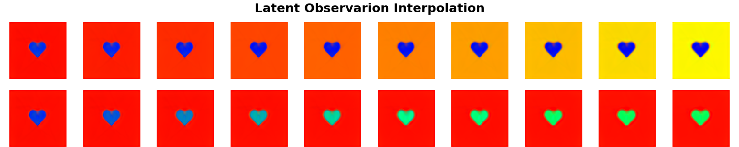
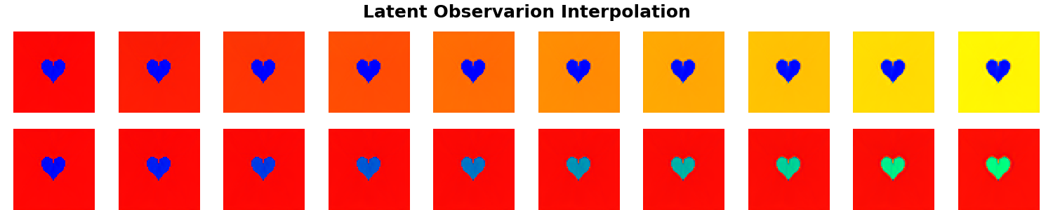
Epochs = 300; $\beta$ = 1

Instead of varying $\beta$, here we vary the number of training epochs. Nonetheless a similar phenomenon is illustrated - depending on how the model is optimised, the learned manifold $\mathbf{z}$ could be disentangled, even though it does not appear as such upon the standard visual inspection following a linear interpolation along the basis vectors.